Entendendo a Resposta Harmônica

A resposta EM de um loop enterrado

\[\begin{split}\frac{H_3^s }{H_3^p} = \frac{\mathcal{E}_3^s }{\mathcal{E}_3^p} = - \frac{M_{12}M_{23}}{M_{13}L} \Big[\frac{\alpha^2 + \imath \alpha}{1+\alpha^2}\Big] \\ = C Q (\alpha)\end{split}\]

Esta expressão tem duas partes. C depende da geometria (coeficiente de acoplamento) e Q depende apenas das propriedades EM do corpo.

• Coupling coefficient: \(C\)

• Response function: \(Q\)

Coeficiente de Acoplamento

O coeficiente de acoplamento pode ser escrito como

\[C = - \frac{M_{12}M_{23}}{M_{13}L},\]

onde \(M_{ij}\) representa a indutância mútua entre os loops \(i\) e \(j\). Derivar a indutância mútua é uma etapa essencial para entender o coeficiente de acoplamento. A indutância mútua pode ser derivada da Lei de Biot-Savart, que nos dá o campo magnético. Suponha que nós estão olhando para dois loops e o campo magnético devido ao primeiro loop é \(\mathbf{B}_1\). Podemos calcular o fluxo \(\Phi_2\) deste campo magnético através do segundo loop da seguinte forma:

(331)\[\Phi_2 = \int \mathbf{B}_1 \cdot da_2 = M_{12} I_1.\]

Este fluxo é então igual à indutância mútua vezes a corrente. Podemos resolver para a indução mútua em mais algumas etapas. Usando o Teorema de Stokes e o potencial de vetor de \(\mathbf{B}_1\), A Equação (331) torna-se uma integral de linha:

(332)\[\Phi_2 = \int \mathbf{B}_1 \cdot da_2 = \int (\nabla \times \mathbf{A}_1) \cdot da_2 = \oint \mathbf{A}_1 \cdot dl_2,\]

onde \(\mathbf{A}_1\) é derivada usando a lei de Biot-Savart:

(333)\[\mathbf{A}_1 = \frac{\mu_0 I_1}{4\pi} \oint \frac{dl_1}{\lvert \mathbf{r} - \mathbf{r'}\rvert^2}.\]

Subpondo a Equação (333) em (332), obtemos a seguinte expressão integral para o fluxo:

(334)\[\Phi_2 = \frac{\mu_0 I_1}{4\pi} \oint \left ( \oint \frac{dl_1}{\lvert \mathbf{r} - \mathbf{r'}\rvert^2} \right ) \cdot dl_2.\]

Podemos então escrever a iduntância mútua entre dois loops como:

(335)\[M_{12} = \frac{\mu_0}{4\pi} \oint \oint \frac{dl_1 \cdot dl_2}{\lvert \mathbf{r} - \mathbf{r'}\rvert^2}.\]

Existem algumas coisa significativas sobre a Equação (335):

Note

• 1- \(M_{12}\) depende puramente da geometria, como o tamanho, forma, e posições relativas dos dois loops.

• 2- Esta expressão não muda se olharmos para o fluxo no primeiro loop devido ao segundo loop, o que significa que \(M_{12} = M_{21}\). Portanto, seguindo os passos da reciprocidade

\[M_{12} = \frac{\Phi_2}{I_1} = \frac{\Phi_1}{I_2}.\]

Efeitos do Coefeiciente de Acoplamento

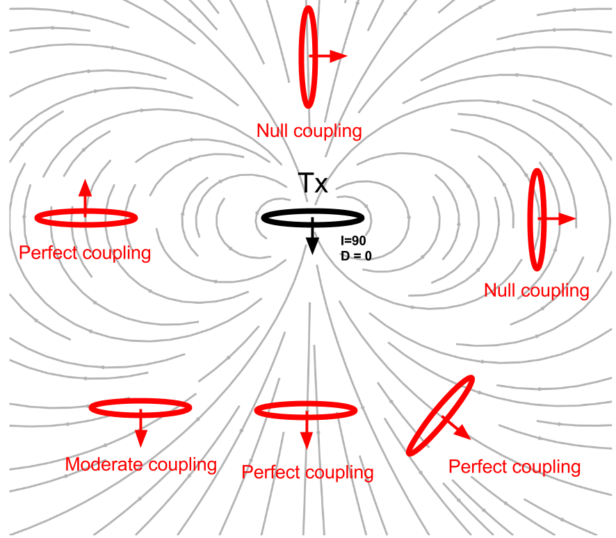
Figura 81 Efeitos do acoplamento entre loops. A orientação dos loops pode ser alterado ajustando a inclinação \(I\) e a declinação \(D\).

Efeitos do coeficiente de acoplamento (\(C\)) muda principalmente devido a orientação dos loops. Nós definimos a orientação de um loop usando inclinação (\(I\)) e declinação (\(D\)) como mostrado em Figura 81. Para definições detalhadas de inclinação e declinação, consulte XXX. Quando o orientação o loop do corpo está alinhado com a linha do campo magnético, melhor acoplamento é criado resultando em maior indutância mútua.

Consideramos uma configuração com três loops: Tx, Rx e corpo. O painel esquerdo de Figura 82 mostra as linhas de campo primárias e a interação entre Tx e Rx e Tx e Body. Conforme mostrado no painel direito de Figura 82, no corpo, o campo magnético secundário é gerado, e tem a mesma direção para \(H^p_3\) em Rx, portanto, a resposta EM (\(H^s_3 / H^p_3\)) tem sinal positivo.

Este processo pode ser explicado por indutância mútua: \(M_ {13}\) terá (-) porque as linhas de campo primárias sobem principalmente em Rx. de forma similar \(M_{12}\) e \(M_{23}\) têm sinais (+) e (-), respectivamente. Portanto, o sinal do coeficiente de acoplamento será positivo. Observe que não apenas o sinal, mas também a decaimento geométrico é considerado na indutância mútua, então como no coeficiente de acoplamento. O coeficiente de acoplamento entre três loops mudará conforme o loop de Tx e Rx se movem ao longo da superfície.

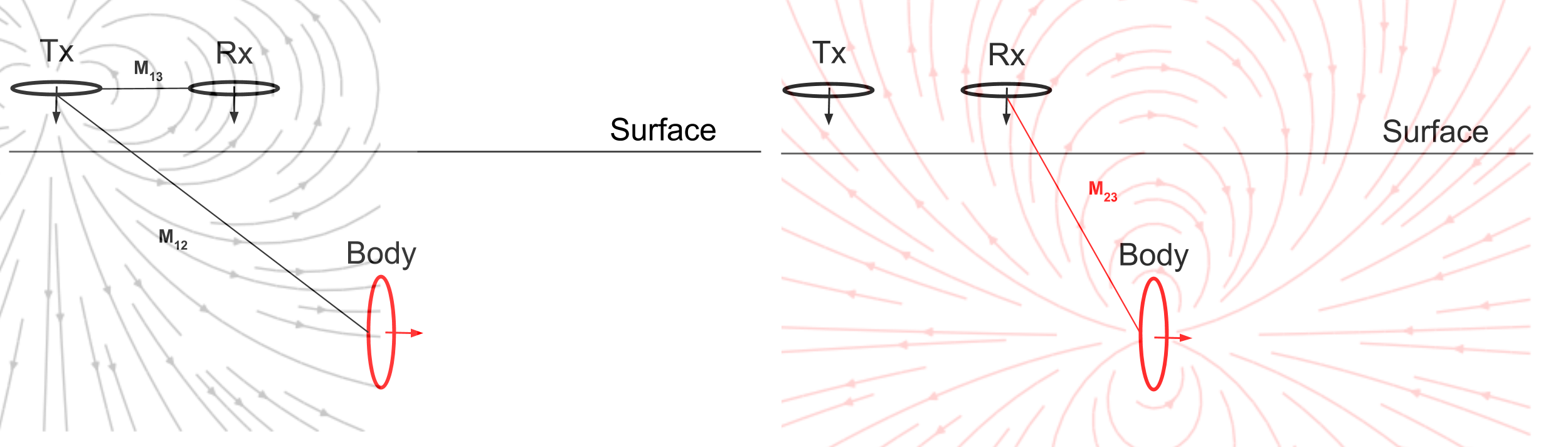
Figura 82 Acoplamento entre 3 loops.

O coeficiente de acoplamento calculado ao longo da linha é mostrado abaixo:

(Source code)

Because the coupling coefficient is generally very small, the EM response, \(\frac{H^s_3}{H^{p}_3}\) is small, regardless of the value of \(\alpha\) [0, 1]. Often part per million (ppm) is used for the unit of this ratio.

Response function

The response function, \(Q\) can be written as

\[Q = \frac{\alpha^2 + \imath \alpha}{1+\alpha^2}\]

Since \(Q\) is complex-valued, we can express them as either real and imaginary or ampliutde and phase.

(Source code)

Asymptotic

We have obtained full expression of the EM response (\(H^s_3/H^p_3\)), which can be written as

\[\frac{H^s_3}{H^p_3} = - \frac{M_{12}M_{23}}{M_{13}L} \Big[\frac{\alpha^2 + \imath \alpha}{1+\alpha^2}\Big]\]

Obtaining asymptotic values of this EM response at small and large \(\alpha\) provides important physical features:

Resistive limit: when \(\alpha \ll 1\):

\[\frac{H^s_3}{H^p_3} \approx - \frac{M_{12}M_{23}}{M_{13}L} (\imath \alpha)\]

The EM response is purely imaginary-valued. The amount of current induced in the body will also be small, and the secondary magnetic field will be everywhere much smaller than the primary field. Therefore, each process of induction(Rx from Tx, body from Tx, Rx from body) can be considered as quite independently.

Note

Within the resistive limit, it is reasonable to superpose EM response from multiple bodies.

Inductive limit: \(\alpha \gg 1\):

\[\frac{H^s_3}{H^p_3} \approx - \frac{M_{12}M_{23}}{M_{13}L}\]

The EM response is purely real-valued, and only dependent of the coupling coefficient. As \(\alpha\) becomes larger, the secondary magnetic field induced an EMF in the body which begins to become appreciable in relation to that induced by the primary field. The phase angle of the current in the body, and therefore the phase angle of the secondary magnetic field, must shift in order that the net induced EMF and the resistive loss should exactly balance. At the inductive limit, this balance virtually becomes equality between the EMFs induced by the primary and by the secondary magnetic field in the body. The induced current and the secondary magnetic field must therefore be in- phase with, but in opposition to the primary field.

Phase

The phase of \(\frac{H^s_3}{H^p_3}\), \(\theta_s\) will be same as that of \(Q(\omega)\), hence

(336)\[\theta_s = - \frac{\pi}{2} - \phi,\]

where

(337)\[\phi=tan^{-1}(\frac{\omega L}{R})=tan^{-1}(\alpha).\]

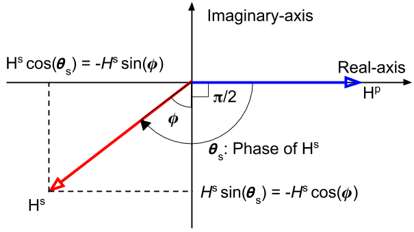
Figura 83 Phase diagram of secondary magnetic field (\(H^s\)).

From above diagram and Eq. (337), it can be seen that:

Note

• For a very good conductor: \(\alpha = \frac{\omega L}{R} \rightarrow \infty\) and \(\phi \rightarrow \frac{\pi}{2}\). In this case, phase of the secondary field is 180 \(^\circ\) (\(\pi\)) behind the primary field

• For a very poor conductor: \(\alpha = \frac{\omega L}{R} \rightarrow 0\) and \(\phi \rightarrow 0\). In this case, phase of the secondary field is 90 \(^\circ\) (\(\frac{\pi}{2}\)) behind the primary field

Assuming the phase of the primary magnetic field, \(\theta_p=0\), its phase lag, \(\psi\), can be written as

(338)\[\psi = \theta_p - \theta_s =\frac{\pi}{2} + \phi,\]

The lag in the phase of \(\frac{\pi}{2}\) is due to the inductive coupling between Loop1 and Loop2, whereas the additional phase lag \(\phi\) is determined by the properties of the conductor as an electrical circuit. That is,

\[ \begin{align}\begin{aligned}H^s_3 = |H^s_3| cos (\omega t - (\frac{\pi}{2}+\phi)) = |H^s_3| sin (\omega t - \phi)\\ = |H^s_3| \Big( cos (\omega t-\frac{\pi}{2}) cos (\phi) + cos (\omega t-\pi) sin (\phi) \Big)\end{aligned}\end{align} \]

The component of \(H^s_3\) 180 \(^\circ\) out of phase with \(H^p\) is \(H^s_3 sin(\phi)\), whereas the component 90 \(^\circ\) out-ouf-phase is \(H^s_3 cos(\phi)\).

In frequency domain EM survey:

• the 180 \(^\circ\) out-of-phase fraction of \(H^s_3\) is called the Real or In-phase component.

• the 90 \(^\circ\) out-of-phase fraction of \(H^s_3\) is called the Imaginary, Out-of-phase, or Quadrature component.