Understanding the response using a widget

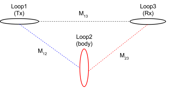
Figura 84 The EM circuit model with three loops.

The EM response from the above circuit model can be written as

\[\frac{H^s_3}{H^p_3} = - \frac{M_{12}M_{23}}{M_{13}L} \Big[\frac{\alpha^2 + \imath \alpha}{1+\alpha^2}\Big]\]

Let I=0 \(^\circ\) and D=90 \(^\circ\) of the Loop2 shown in Figura 84. For this case, we consider a loop-loop EM survey with the geometry of EM-31 (3.66m Tx-Rx offset), and the body (Loop2) is embedded 3 m below the surface. Figura 85 shows complex response function (Plot1), easting line at 0 m-northing (Plot2), plan maps of real and imaginary part of the EM data with the loop-loop EM survey when \(\alpha\) =0.31. Plot2 clearly shows how coupling is changing depending on relative location and orientation of three loop system. Plot3 and Plot4 illustrate plan map of EM data we could possibly obtain by acquring multiplie lines. Following considers different orientation of the body (Loop2), which will generate different coupling effects on the measured EM data.

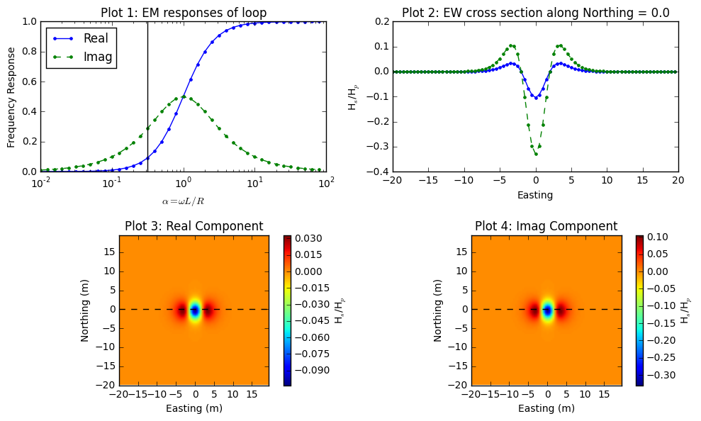
Figura 85 Frequency domain EM response from loop-loop EM survey when I=0 \(^\circ\) and D=90 \(^\circ\).

Figura 86 shows same figures, but with different I and D of body (Loop2): I=-90 \(^\circ\) and D=0 \(^\circ\). Shape anomalous response is significantly different due to the different coupling among three loop system. Especially, the peak anomaly at the center has positive sign. Figura 87 shows the case when I=0 \(^\circ\) and D=0 \(^\circ\). This is null-coupled case where there is no primary flux passing the area of Loop2, hence measured reponse is zero everywhere.

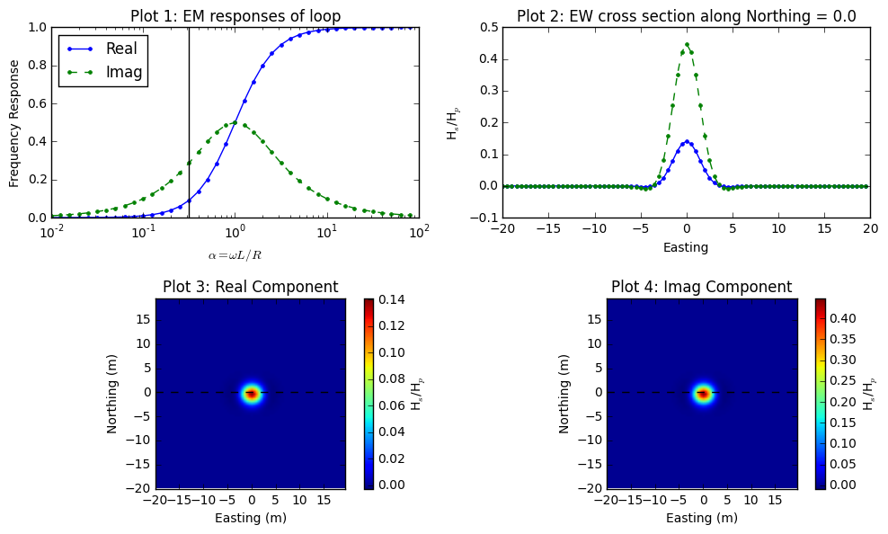
Figura 86 Frequency domain EM response from loop-loop EM survey when I=-90 \(^\circ\) and D=0 \(^\circ\).

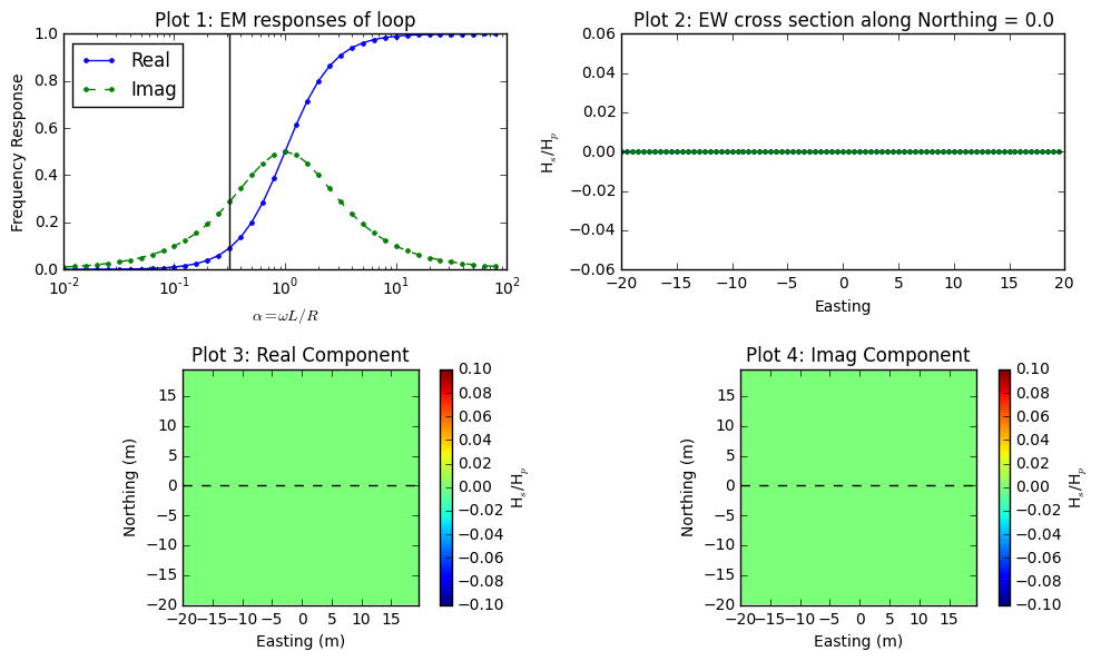
Figura 87 Frequency domain EM response from loop-loop EM survey when I=0 \(^\circ\) and D=0 \(^\circ\).

If you want to play with loop-loop EM survey click below: